

Blog
The Best Indoor Air Quality Monitors
Indoor air quality can have a major impact on the comfort and productivity of homes, offices, schools, laboratories, and industrial facilities. Carbon dioxide buildup, poor






Conductivity temperature compensation is the correction of the electrical conductivity (EC) for temperature variations. This allows readings to be standardised to a reference temperature so that differences between readings can be compared to ion concentration rather than thermal effects.
If you’ve been comparing conductivity measurements taken at different temperatures without temperature compensation, your conclusions may be misleading. Electrical conductivity (EC) tells you how readily a solution carries an electrical current. This ability comes entirely from dissolved ions. When a voltage is applied across the two electrodes, the ions migrate. When you measure how much the current flows, normalise the electrode geometry, and you have your conductivity level, in Siemens per centimeter.
The physics are well understood, and have been for over 100 years. The complication isn’t the measurement of conductivity itself. The challenge is that ions don’t move through water the same way they do at 10℃ (50℉) as they do at 30℃ (86℉). This difference in temperature is large enough to matter in almost every application where conductivity is monitored.
Simply, water viscosity drops when the temperature rises. When water (or a solution) has lower viscosity, it causes less drag on the ions as they move through the solution. Less drag results in ions moving faster, and faster-moving ions carry more current. If the solution experiences more current, it means your conductivity sensor reports a higher conductivity. So, even if the chemical composition of the solution remains unchanged, a change in temperature can produce a noticeable change in measured conductivity.
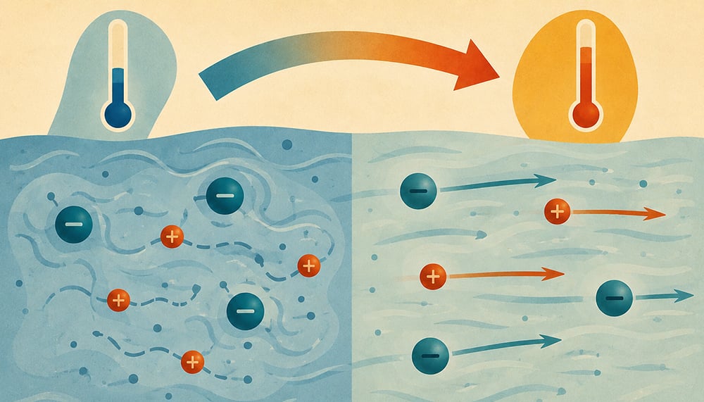
As a solution cools, ions lose kinetic energy, and their movement through the liquid slows. The slower the ions move, the less current there is flowing across the electrodes. That reduces the conductivity ( and increases the resistivity ) . On the other hand, by heating a solution, the ions become more mobile and the conductivity increases.
This behaviour can be observed even in standard calibration solutions. Calibration of the conductivity and determination of the cell constants are often performed using standards of potassium chloride (KCl) whose conductivity is a predictable function of the temperature change. Allowing both ion concentration and temperature to vary simultaneously would make the interpretation of conductivity readings unnecessarily hard. If the temperature is held constant, or mathematically corrected for, the changes in conductivity are isolated to the variable that usually matters most: the ion concentration. This is precisely why temperature compensation is such a critical feature of conductivity measurement systems.
Conductivity measured without correction for temperature is often called absolute conductivity or uncompensated conductivity. In most practical systems, measurements are corrected to a standard reference temperature, usually 20 or 25 °C. To do this, the instrument measures the temperature of the solution and applies a compensation factor that describes how strongly the conductivity responds to a change in temperature. This factor is often called beta (β), or the temperature coefficient.
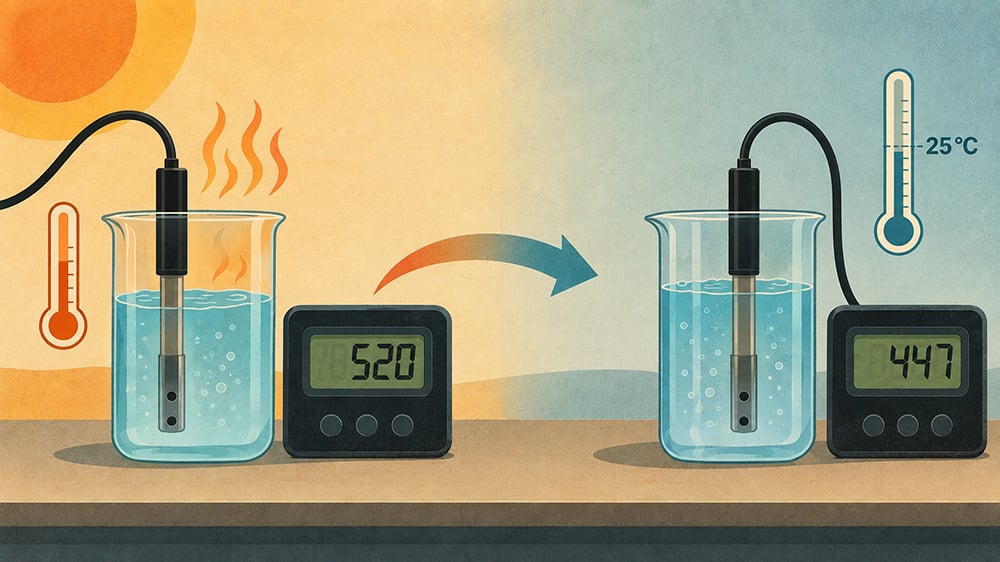
For many neutral salt solutions, β is generally 1.5–2.2% per °C, which is why the popular 2% per degree rule works reasonably well in many aqueous systems. More advanced conductivity instruments can allow the user to adjust β for different chemistries and select a custom reference temperature when 25 °C is not appropriate.
As mentioned, the practical magnitude of this effect is approximately 2% per degree Celsius for most aqueous solutions. For example, a nutrient solution sitting inside a greenhouse may be 16℃ (60.8℉) in the morning when the sun is weaker, but by the afternoon it could creep up to 26℃ (78.8℉). That is a 10℃ shift. Uncompensated, you would likely see 20% more conductivity when the temperature is warmer, compared to measurements taken in cooler temperatures. This all happens to the same solution despite not adding any dissolved solids; it is all down to temperature. If you have an automated dosing system running on those raw readings, you would spend the day chasing a problem that doesn’t exist.

This is the core of why temperature compensation exists. It doesn’t just make your measurements more accurate, but it also makes them consistent.
The standard linear compensation model is pretty simple. You take the raw conductivity reading, the sample temperature, the reference temperature, and a coefficient that explains how sensitive your solution is to temperature. You can use the following:
EC_compensated = EC_measured / [1 + α(T – T_ref)]
The reference temperature across industries and applications is almost universally 25℃. This is what most calibration standards are certified at, and that is the temperature where sensor manufacturers anchor their reported values. The alpha coefficient (α) is where things start to get interesting.
Alpha is not a universal constant, as it depends on which ions are in a solution and how they react with the concentration of the solution. In natural water and freshwater applications, alpha values close to 0.019 are often used. Solutions containing sodium chloride typically sit closer to 0.020, and saltwater is somewhat lower. And concentrated acids and bases can deviate a lot from any of these figures.
The temptation is to use the default of 2%, and for some applications, rough process monitoring and basic water quality screening, it can be acceptable. But if you are running pharmaceutical buffers, USP purified water, precisely formulated nutrient solutions, or a solution with unusual ionic composition, using a generic alpha can present systematic error that travels through your dataset. For example, the compensation may appear to be working as the numbers are changing, but they may be changing to incorrect values.
When accuracy is key, determine alpha empirically for your type of solution by measuring the conductivity value across several controlled temperatures – this fits the appropriate relationship. It doesn’t take too long, but it is important.
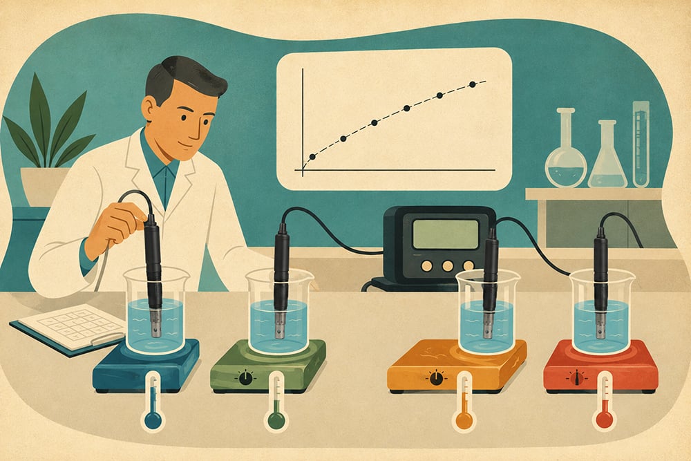
The linear formula remains strong between 15℃ and 35℃ in many ionic solutions. But if you push outside of that window, or you are working with chemically complex fluids, the approximation starts to weaken.
If we were to take ultrapure water (typical conductivity of 0.55 μS/cm – microSiemens per centimeter), the ion concentration from dissolved salts is minimal. What you are measuring instead is conductivity stemming from water’s own autoionization.
The equilibrium constant for this reaction is strongly temperature-dependent and non-linear. Near room temperature, conductivity changes in ultrapure water cannot be reliably approximated using a single fixed alpha over a broad temperature range. So, the correct approach for ultrapure water is to use tabulated correction factors or non-linear compensation models from theoretical and empirical conductivity relationships. Most laboratory-grade conductivity meters have this type of compensation embedded.
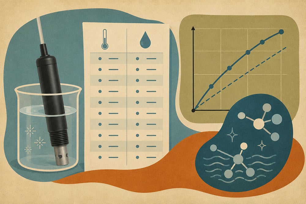
Similar deviations from linearity can also occur in very concentrated solutions where ion-ion interactions become increasingly important, and the simple linear mobility assumption no longer holds. In these systems, empirical models or chemistry-specific compensation schemes are often better than generic coefficients. If your application falls into this region, it’s worth asking the instrument manufacturer what compensation algorithm is really running under the hood. “Temperature-compensated” on a spec sheet can mean anything from a chemistry-specific model to a hard-coded 2% linear correction.
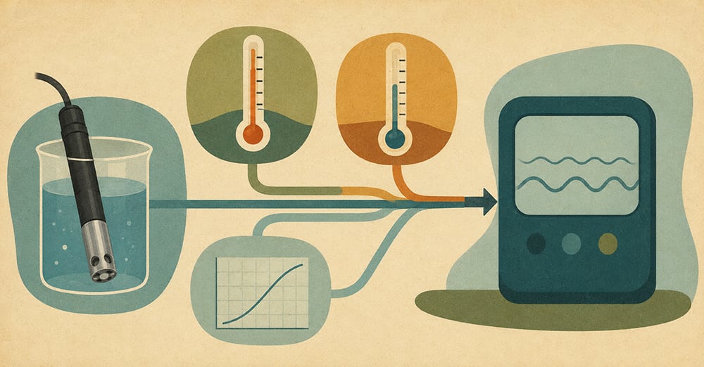
Good compensation math is worthless without accurate, real-time, co-located temperature data. This is where good intentions often fail in practice, often because the conductivity probe was not as well thought out as the temperature sensor.
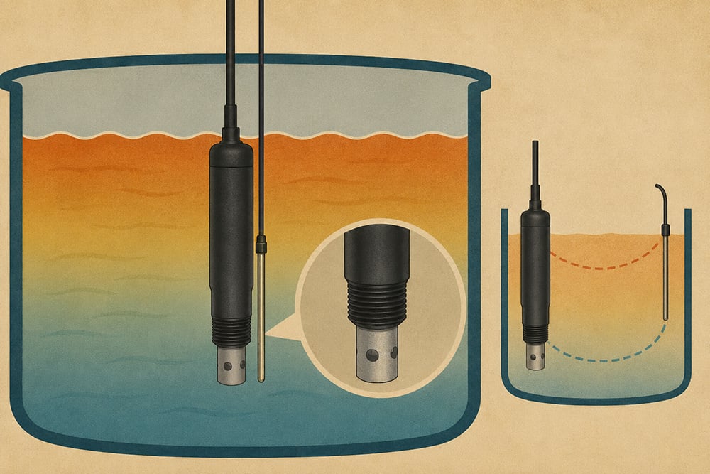
The temperature sensor should be positioned as close as possible to the conductivity electrodes. In a stratified tank, poorly mixed reactor, or any system with spatial temperature gradients, a sensor mounted even a few centimeters away may actually be measuring a meaningfully different temperature than the fluid in contact with the electrodes. For a solution with a temperature coefficient near 2%/°C, a 2–3 °C temperature mismatch could introduce roughly 4–6% error into the temperature correction. This is enough to lose much of the compensation benefit in many systems.
Response time is also important, especially in dynamic environments. If your conductivity probe equilibrates to a new temperature in 2 seconds, but your temperature sensor takes 10 seconds, then you are applying yesterday’s temperature to today’s conductivity, or at least the temperature from several seconds ago. In steady-state systems, this doesn’t matter too much. This can be a major source of measurement error in flow-through cells, outdoor deployments, or rapidly changing process streams.
Platinum RTD sensors, in particular the PT-1000, are widely used in precision conductivity systems. Their resistance-temperature relationship is stable and reasonably linear over typical operating ranges. Thermistors, on the other hand, often respond faster and cost less, but their stronger non-linearity and greater device-to-device variation can make calibration more challenging. Therefore, overall system performance doesn’t just depend on the type of temperature sensor, they also depends on thermal coupling, calibration quality, electronics, and installation geometry.
Temperature compensation and calibration interact in ways that catch a lot of people out. The values on conductivity calibration standards are only strictly valid at that temperature. For example, if you were to pour the standard into a beaker and let it sit in a warm room, then calibrate it immediately without allowing thermal equilibrium, you would risk offsetting the calibration.
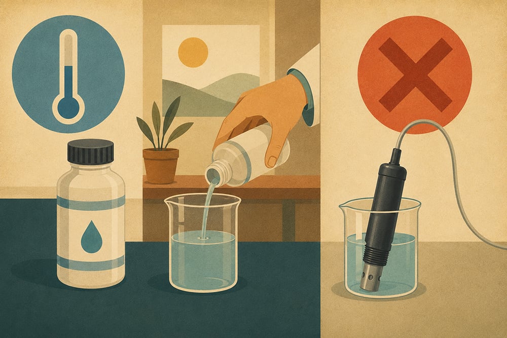
Most modern conductivity meters compensate for temperature during calibration and measurement. But if the probe has not equilibrated, or if the wrong temperature reference is used, the baseline can shift. To fix this, let the probe and standard equilibrate fully before accepting the calibration point.
The same logic applies to calibrating in the field. High-quality conductivity standards often include temperature-conductivity tables for this precise reason. When they are available, use the value appropriate to the actual calibration temperature rather than assuming.
One of the best habits to get into is logging the raw, uncompensated conductivity, the sample temperature, and the compensated conductivity. The reason is that if you later find that your alpha coefficient was incorrect, the compensation algorithm changed after a firmware update, or your temperature sensor had an offset, you can easily go back and recalculate from the raw data in the log.

In regulated industries, this is essential in case data needs to be recovered after a failed audit trail. This can also prevent the need for repeating an entire experiment.
The relationship between compensated and raw conductivity across temperature can also reveal issues such as emerging sensor failure, cell constant drift, and probe fouling. These problems may stay hidden if you are only chasing the final compensated number.
Conductivity temperature compensation is a mathematical correction applied to EC measurements in solutions. It requires an alpha coefficient, sensor placement, and calibration protocol.
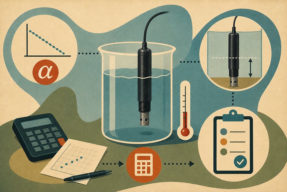
If you need help with conductivity temperature compensation in your solution, or you are unsure which conductivity and temperature probe is best for your application, do not hesitate to contact the world-class team at Atlas Scientific.

Indoor air quality can have a major impact on the comfort and productivity of homes, offices, schools, laboratories, and industrial facilities. Carbon dioxide buildup, poor
UART and I2C are serial communication protocols, but they serve different purposes. UART is typically used for direct device-to-device communication and requires dedicated connections. I2C